Building a Recommendation System with Deep Learning and TensorFlow

1. Before We Begin

Hello, I’m Mike (Sanghoon Kwak), product manager for content and machine learning at Buzzvil, a mobile lockscreen ad network. Buzzvil uses deep learning to recommend personalized content automatically, improve the user experience, and maintain a technological edge as an advertising platform. In this post, I’ll share how we developed that recommendation logic and the results we achieved. I assume a basic understanding of neural networks, keep code to a minimum, and focus on the model’s high-level design. Links throughout provide more detailed formulas, proofs, examples, and code.

2. Background

Only ten years ago, commonly used AI techniques still fell short as general-purpose machine learning tools. One reason was the lack of automatic feature selection. Systems depended heavily on hand-crafted features created by specialists for particular tasks, such as morphological analysis for natural language processing or edge detection for image recognition. Neural networks—or deep learning—have recently returned to prominence because automatic feature learning addresses this problem, making them better suited to learning across different domains. They have drawbacks: their black-box nature makes them hard to interpret intuitively, training takes time, and parameter tuning requires considerable effort. Yet their effectiveness in pattern recognition is already well established (see http://karpathy.github.io/2015/05/21/rnn-effectiveness/). When I first encountered RNNs, I fed the ten volumes of Lee Moon-yeol’s Romance of the Three Kingdoms into an experiment on my MacBook similar to those in the linked article. The output was surprisingly plausible—the quotation marks, question marks, and exclamation marks were especially well placed.

Hearing those words, Cao Cao asked Yuan Shao in response to Yuan Shao’s words. “You said this without anywhere. Unless you turn beneath these words, there is something that will surely try to kill those soldiers. This time, together with Yuan Shao, how else are we to strike them and do one thing!” Hearing those words, Cao Cao asked again. “We all have military provisions, so which thing is today?” Yuan Shao spoke as Cao Cao answered that way. “What does this person mean?”

“We are killing soldiers like that place and listening to those words. It is already that.”

With that introduction out of the way, let me explain the recommendation system we built at Buzzvil using this powerful tool.

3. Application

Slidejoy, Buzzvil’s service in the United States and Europe, offers users a variety of lockscreen content alongside ads. Every hour, it stores and cleans more than 10,000 articles from over 200 content providers and presents them to users by category (see https://techcrunch.com/2016/01/28/lockscreen-app-slidejoy-gets-a-newsy-new-feature/). Initially, before introducing neural networks, we grouped content using a simple unigram TF-IDF approach and showed everyone the same topics, ordered by how frequently they were mentioned.

[Image source: TechCrunch, January 2016, Lockscreen App Slidejoy Gets A Newsy New Feature]

We then saw a need to offer content tailored to individual interests, beyond topics that were popular with everyone, and began developing personalization with deep learning. We used Google’s TensorFlow, which was seeing rapid adoption, for all of this work.

4. Model Design

1) Data collection: The data collected through Slidejoy’s content service falls into three main groups.

• Basic user data: user ID, gender, age, and similar information.
• Content data: category, provider ID, title, description, and so on.
• User interaction data: display order, time, and whether the user clicked.

To make the data easy to use as TensorFlow training input, we stored it in daily TFRecord files (see https://www.tensorflow.org/api_docs/python/python_io/#tfrecords_format_details). We used three months of data for initial training.

2) Model components: In TensorFlow, you first construct a graph that defines the data flow, from input through backpropagation, using tensors—think of them simply as vectors—to hold the data. When defining the graph, all tensor operations must use TensorFlow functions (see https://www.tensorflow.org/api_docs/python/array_ops/). Ordinary NumPy or list operations do not become part of the graph. After defining it, you start a session and let actual data flow through an operation in the graph to perform learning. Hence the name “TensorFlow.” If you are new to machine learning, this development style may feel unintuitive, but it makes the underlying graph very convenient to save, load, and inspect.

• Objective

The basic goal of content recommendation is to order items according to a user’s preferences. Preferences can be defined in many ways; for this project, we used whether the user clicked an item. Given user and content information, the neural network ultimately predicts the probability of a click.

• Input

We used TensorFlow’s shuffle_batch function to shuffle the daily training datasets before feeding them into the model. As mentioned earlier, the input files are TFRecords; their binary format is much faster than ordinary CSV or text files. TensorFlow batching uses queues and dequeue operations (see https://www.tensorflow.org/how_tos/reading_data/). The steps are:

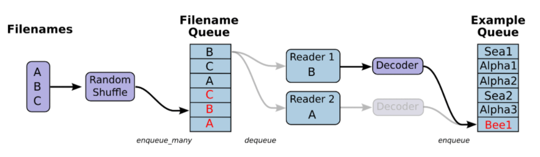
[Image Source: TensorFlow, 'Reading Data']

1. Add the required filenames to a filename queue with tf.train.string_input_producer.

filename_queue = tf.train.string_input_producer(files)

2. Read files dequeued by the input producer with a reader appropriate to the format, such as CSV or TFRecord, and add the resulting examples to another queue.

reader = tf.TFRecordReader()
_, serialized_example = reader.read(filename_queue)

3. Use shuffle_batch or batch to dequeue examples and feed the actual data into the graph.

features = tf.train.shuffle_batch(
   tensors=[serialized_example],
   batch_size=batch_size,
   capacity=capacity,
   min_after_dequeue=min_after_dequeue,
)

4. Data can be fed only into placeholders. Define the placeholders that will receive it when creating the graph.

# placeholder 들 생성 
label = tf.placeholder(tf.int32, [None, ], name='y-input')

...

# queue runner 시작 및 feature 추출 
sess = tf.Session()
coord = tf.train.Coordinator()
threads = tf.train.start_queue_runners(sess=sess, coord=coord)
features = sess.run(features)

# Cost/loss 계산을 위해 batch output 을 placeholder 들에 feed 
feed_dict = {
    label = features[0].values, 
    ...
}

# feature 를 이용해서 cost 계산 
sess.run(cost, feed_dict=feed_dict)

If you read and write TFRecords, I strongly recommend replacing the Python-based protobuf library used by TensorFlow with its C++ implementation. It can be 10–50 times faster (see https://github.com/tensorflow/tensorflow/blob/master/tensorflow/g3doc/get_started/os_setup.md#protobuf-library-related-issues).

• Embeddings

We embed all sparse features, including user IDs, content category IDs, user ages, and times. An embedding is essentially a lookup table or matrix that projects sparse data into a dense, high-dimensional vector space. Define the embedding matrix as a variable, and learning updates it alongside the network’s weights. Remarkably, similar features then cluster together in that vector space. TensorFlow provides embedding lookup functions (https://www.tensorflow.org/api_docs/python/nn/embeddings), making embeddings easy to apply.

embeddings = tf.get_variable(
   'embedding',
   initializer=tf.random_uniform([size, dimension], -1.0, 1.0)
)

y = tf.nn.embedding_lookup(embeddings, feature)

For words in content titles and descriptions, however, we use a pretrained constant matrix (tf.constant) rather than a variable. Many word embedding matrices have already been trained on documents from Wikipedia, Twitter, and other sources. Using one saves us the work of training a new embedding. Specifically, we chose Stanford’s Wikipedia + Gigaword embeddings. The methodology is explained at http://nlp.stanford.edu/projects/glove/. As that reference shows, words appearing together in similar contexts lie near one another in vector space, and even simple vector arithmetic works: v_king - v_queen ~= v_man - v_woman.

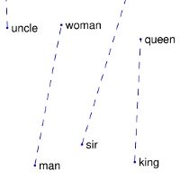
[Image Source: Global Vectors for Word Representation]

• Hidden layers: We used two main kinds of hidden layer.

1. RNN layer We applied an RNN to the sentence features—the content title and description. Before settling on this, we experimented with CNNs, more commonly used for image recognition, and unidirectional RNNs. A single bidirectional RNN layer performed best. We used long short-term memory (LSTM) cells to address the vanishing and exploding gradient problems of basic RNN cells (see http://colah.github.io/posts/2015-08-Understanding-LSTMs/). TensorFlow has two main RNN variants: static and dynamic. Dynamic RNNs construct the graph when the session executes, making initial graph creation much faster. However, as the documentation explains, a static RNN can stop early according to the sequence length rather than compute every time step. For example, an embedded title matrix with a total dimension of 100 would normally require 100 RNN steps. If a short title has a sequence length of 5, computation stops after the fifth step, saving work.

A dynamic RNN, by contrast, does not stop early; it pads the output after the specified sequence length with zeros. The two functions also have different input specifications, so take care when using them.

Initial graph creation was not particularly slow in my case, so I used a static RNN.

def lstm_cell(layer_size):
   return tf.nn.rnn_cell.LSTMCell(
       num_units=layer_size,
       forget_bias=1.0,
       state_is_tuple=True
   )

outputs, final_state_fw, final_state_bw = tf.nn.bidirectional_rnn(
   cell_fw=lstm_cell(layer_size),
   cell_bw=lstm_cell(layer_size),
   inputs=input,
   dtype=tf.float32,
   sequence_length=sequence_length
)

2. Feed-forward layer We concatenate the RNN output with all the embedded inputs, then pass the result through a multilayer network to produce a final two-dimensional output: click or no click. I used Xavier weight initialization, which preserves input variance and prevents weights from causing inputs to vanish or become excessively amplified (see http://jmlr.org/proceedings/papers/v9/glorot10a/glorot10a.pdf). It is especially useful in networks with many layers.

• Cost Function

The neural network has a final output dimension of two. We apply softmax to turn it into a probability distribution. Softmax is the most common transformation for converting arbitrary vector values into probabilities. Its formula below gives the probability of category c from output vector z.

 

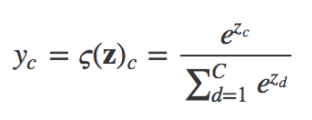
We calculate loss, or cost, using the cross-entropy between these probabilities and the actual click labels. The formula follows, where y is the label and a is the probability.

We chose cross-entropy over mean squared error, (y - a)^2, to address the shrinking gradient—and therefore slower learning—as probabilities approach 0 or 1. That is why cross-entropy is commonly used for classification (see http://neuralnetworksanddeeplearning.com/chap3.html).

TensorFlow conveniently combines softmax and cross-entropy in one function, softmax_cross_entropy_with_logits (see https://www.tensorflow.org/api_docs/python/nn/classification).

3) Evaluation and monitoring Training loss indicates whether a model is converging, but a more intuitive metric is needed to understand its practical effectiveness. For classification, accuracy is usually computed by comparing the highest-probability category—the softmax result—with the actual label. If the test or evaluation results look like this, 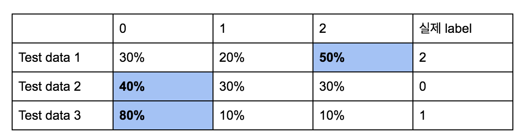accuracy would be 66.6%. For content clicks, however, more than 90% of examples are 0, or no click, so this accuracy metric is not very informative. We instead used AUC, area under the curve, to evaluate the relationship between predicted click probabilities and observed clicks despite this imbalance. For a detailed definition, see http://www.dataschool.io/roc-curves-and-auc-explained/. Briefly:

• Plot the true-positive rate against the false-positive rate at different thresholds, then calculate the area under that curve.
• We have predicted click probabilities (p_1, p_2, p_3, ... , p_n; 0 <= p_x <= 1) and their corresponding categories (c_1, c_2, c_3, ... , c_n; c_x = 1 or 0).
• If every pair (p_x, p_y) with p_x > p_y also has c_x > c_y, AUC is 1.
• Conversely, if every such pair has c_x < c_y, AUC is 0.
• Random probabilities generally give an AUC around 0.5, so a value above 0.5 tells us the predictions contain useful information.

For convenience, we calculated AUC using sklearn’s function (see http://scikit-learn.org/stable/modules/generated/sklearn.metrics.roc_auc_score.html).

4) Tuning

• Overfit

When training repeatedly on the same data, training cost often continues to fall while evaluation or test cost does not. The model is overfitting the training data. There are several ways to address this.

Data: A simple and highly effective approach is to increase the amount of training data!

L2 regularization: This prevents weights from becoming too large. At a high level, large weights make outputs swing more strongly with the inputs, potentially fitting noise rather than general patterns and making the model less generalizable.

# weight 를 이용한 l2 regularization 
for weight in weights:
    cost += l2_reg_lambda * tf.nn.l2_loss(weight)

Dropout: A simple and highly effective approach is to increase the amount of training data!

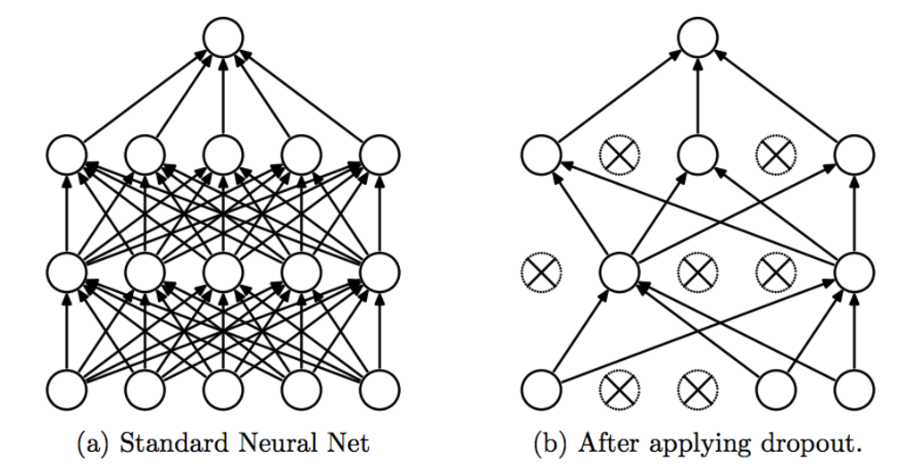
[Image Source: A simple way to prevent neural networks from overfitting]

As the illustration shows, training randomly removes nodes with a fixed probability. At a high level, using a different random subset of nodes each time has an effect similar to training several models and averaging them. Like regularization, this helps produce a more generalizable model.

 

• Tensorboard

There are many ways to monitor training once the model is designed, but TensorFlow’s TensorBoard is the easiest. It lets you track changes in weights and biases, accuracy, and cost at every iteration. I found its graph visualization particularly useful: it clearly organizes data dimensions, flow, and the variables being trained (see https://www.tensorflow.org/versions/master/how_tos/graph_viz/).

To use TensorBoard:

While defining the graph, record summaries for the scalar values you need, then merge them.

tf.scalar_summary(‘cost’, cost)
...
merged = tf.merge_all_summaries()

After creating the session, define a summary writer.

Writer = tf.train.SummaryWriter([directory], sess.graph)

Retrieve the summaries at each iteration.

summary, ...  = sess.run([merged, ... ], feed_dict=...)
writer.add_summary(summary, step)

• Parameter optimization

Many parameters can be tuned: learning rate, batch size, dropout rate, L2 regularization rate, and more. There is no formula for finding the right values. Make changes, monitor convergence speed and AUC continuously, and work toward better settings. It is more art than science.

After designing the model, we trained it for about 100 epochs on three months of data. Each evaluation dataset contained one user’s content consumption over a week. Because users have different click probabilities, we did not mix multiple users when evaluating results. Naturally, evaluation data was excluded from training. Toward the end of training, evaluation AUC was consistently around 0.7. Once satisfied with that result, we used the model to serve personalized content to real users and measured the improvement in click-through rate.

5. System

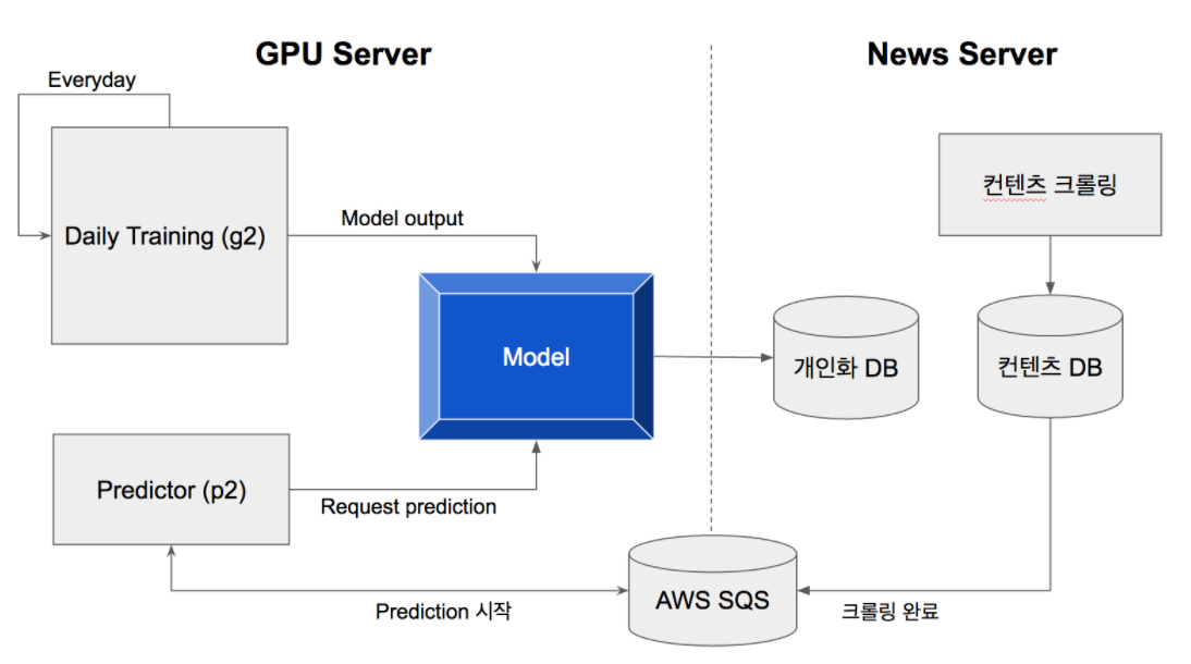Deploying the model in Slidejoy involved two main components: daily training and prediction.

• Daily training runs continuously, using only the most recent 60 days of data. At the end of each day’s training, we transfer the model parameters to a p2 instance. Retraining on all historical data would take too long, and user preferences can change over time. We used an AWS g2.2xlarge instance for training. AWS offers two main GPU instance families, g2 and p2. The p2 is about 40% more expensive but has a more powerful GPU, with three times the GPU memory, three times the processing cores, and other improvements. In this project, a p2.xlarge processed each iteration about 40% faster than a g2.2xlarge.

• Prediction is time-sensitive, so we used the faster p2.xlarge instance. When content collection finished, we sent a completion message to AWS SQS. On receiving it, the prediction instance calculated probabilities for more than 10,000 content items for each of 3,000 test users every hour, storing the results in Redis.

6. Results

To evaluate the model, we ran an A/B test with 3,000 active Slidejoy content users, divided into three groups.

• Group A: Random content.
• Group B: The same content for everyone, with articles grouped using unigram TF-IDF and ordered by topic popularity.
• Group C: Personalized content ordered by the neural network’s predicted click probability for each user.

After two weeks, we had enough impressions and clicks to evaluate the results. Group B’s click-through rate was 22% higher than Group A’s, and Group C’s was 25% higher than Group B’s; both differences were statistically significant. Even this simple model produced meaningful results in a real application.

7. Closing Thoughts

This project began with content personalization, but Buzzvil plans to apply neural networks rapidly to ad targeting, revenue growth, operational automation, marketing, and other areas. As noted at the start, neural networks reduce the need to hand-design domain-specific features, allowing a generalized model to serve multiple purposes. Our next step is therefore to build a generalized model and system that can accept different kinds of data and make different kinds of predictions. We might add specialized layers or omit unnecessary ones as needed, like Lego bricks. The recommendation model described here is, as mentioned, fairly simple. Looking at the model behind Google Translate’s recent, well-received move to neural networks is humbling (see https://arxiv.org/abs/1609.08144). There is plenty of room for improvement as we pursue our longer-term goals.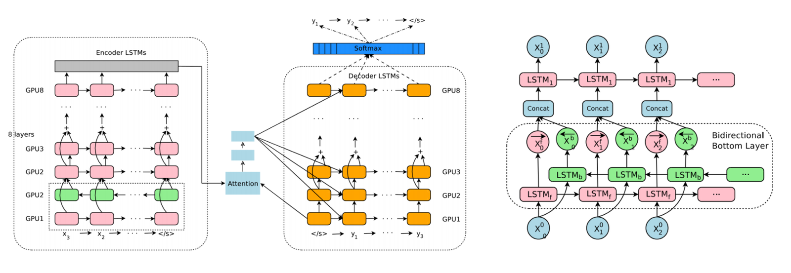

[Image Source: Google's Neural Machine Translation System]

1. Parallel Architecture

As the design above and its reference explain, only one bidirectional RNN layer is used—even though bidirectional RNNs outperform unidirectional ones—to maximize model parallelism. Once the first time step of one unidirectional RNN layer finishes, the next RNN layer can immediately calculate its first time step. A bidirectional layer, by contrast, must complete all time steps before the next layer can proceed. This makes it possible to calculate multiple RNN layers in parallel across multiple GPUs.

Data parallelism matters alongside model parallelism. It runs multiple models simultaneously and has them update one shared set of model parameters.

As mentioned earlier, finding optimal parameters and important features requires many experiments. We need to run as many of them as quickly as possible, and these parallel architectures will help us build a better model.

2. Automated tuning

We need experiments that remove features and monitor the resulting metrics to identify which features matter, then emphasize the important ones. For example, if including content titles significantly raises AUC, we could make the title RNN more complex so it better understands context. Parameters such as learning rate, regularization rate, and dropout rate also need experimental optimization. Designing a system that automates much of this work will be central to building a generalized model.

3. Reinforcement Learning

Beyond supervised learning, many neural-network reinforcement learning models have been published, including DQN and A3C. They have mainly been applied to games with relatively small, well-defined state spaces, but they may also work well for ad and content allocation policies.

4. TFlearn (http://tflearn.org/)

I used TensorFlow’s functions directly for this project, but there is a simpler library: TFLearn. It packages repetitive graph-construction operations—creating placeholders, defining weights and biases, applying regularization and dropout—into higher-level functions.

Specifying tensor dimensions and reshaping tensors as needed is tedious and error-prone. TFLearn handles these repetitive operations cleanly. For example, the following two lines create a feed-forward layer with weights, biases, activation, regularization, and dropout all included.

dense1 = tflearn.fully_connected(
    input_layer, 
    64, 
    activation='tanh', 
    regularizer='L2', 
    weight_decay=0.001
)

dropout1 = tflearn.dropout(dense1, 0.8)

We still need to investigate its performance and correctness, but it looks well suited to reducing mistakes, learning TensorFlow, and implementing simple models. I’m excited to see how further deep-learning and neural-network research will change Buzzvil’s services.